
A/B Testing and Econometrics - Part 2
Published:
This is the second post in a two part post on A/B testing and causal inference using Econometric methods. The first post can be found here.
At the end of the last post I made a case of why Econometric techniques could come in handy when A/B testing can’t be carried out. This post will deal with an explanation of what these Econometric techniques for causal inference are.
These techniques and examples may seem very specific to just questions that economists ask. But, if you really think about it from a statistical perspective these techniques to establish causal inference are broadly generalizable to other contexts as well, such as in a product setting where A/B testing isn’t feasible.
Difference in Difference
Among other things, the primary condition that is required for causal inference is an accurate counterfactual that can act as the control. A counterfactual is the what if condition - it answers the question of what would have happened if the treatment had not occurred. In an experimental setting the control group performs this role.
The difference in difference method exploits what economists call a ‘natural experiment’ to construct this counterfactual. This works by identifying two similar groups, one that is randomly affected by the treatment and one that is not affected by the treatment. The group that is not affected by the treatment serves as the counterfactual for the group that is affected by the treatment. The difference between the effect on the group affected by the treatment and what would have happened if the same group wasn’t affected by the treatment is the causal effect of the treatment. The ‘what if’ scenario is constructed using the counterfactual.
A classic case where this is used in economics is in evaluating the causal effect of policy changes. It is often the case that policies are enacted on a state level, this results in the state where the policy change is enacted acting as the treatment and the neighbouring state or a demographically similar state acting as the control.
This can visually be illustrated easily using the following picture: 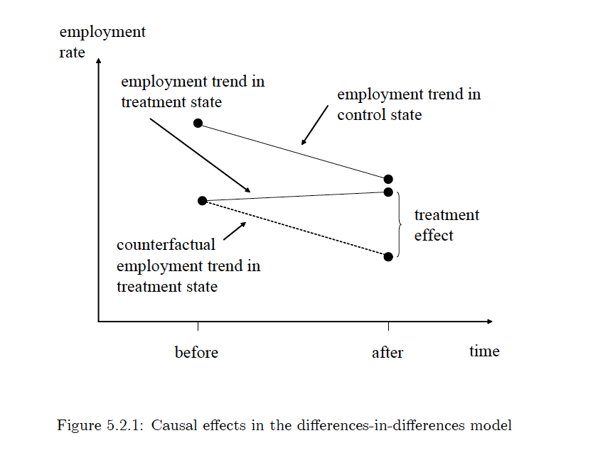
Source: Mostly Harmless Econometrics An Empiricist’s Companion by Joshua Angrist and Jorn-Steffen Pischke
Given the fact that this is an experiment that has not been constructed, it makes one big assumption. The fact that both groups, in the absence of the random treatment, would behave in the same manner over time. This is known as the ‘parallel trends’ assumption. While exploiting a natural experiment to construct a difference in difference study, it is crucial to try and validate this assumption.
In addition to this, the difference in difference can also be modeled using a regression framework. In this case, the independent variable is the metric of interest and the dependent variable is a dummy variable that takes on a 0 for when the treatment doesn’t exist and 1 for when the treatment exists. The advantage of this design is two-fold. First, this allows for multiple states or groups that serve as both control and treatment, as long as the introduction of the treatment is randomly varied across time. Second, it allows for the controlling of confounding variables. Confounding variables are other things independent of the treatment that can affect the dependent variable. Controlling for these factors strengthens the statistical significance of the causal interpretation.
Instrumental Variables
In a non experimental setting an important consideration when it comes to causal inference is the omitted variable bias. Omitted variables are variables that a regression setup does not account for that are captured by the error term. This breaks down a key assumption of causal inference that the independent variables and the error term must be uncorrelated.
A classic example from economics is estimating the effect of schooling on wages. In addition to schooling, wages are also influenced by the ability of an individual which is likely correlated with the amount of schooling an individual receives. Students with higher ability who do better at school tend to stay longer in school. If wages are regressed on schooling, the error term would likely represent ability and cause the estimate of the effect of schooling on wages to be off. In other words, the error term will be correlated with the dependent variable.
The tool that economists use to correct this is called the Instrumental Variable, sometimes just referred to as the Instrument. The idea is pretty simple: it requires the identification of a dependent variable that is correlated with the original dependent variable of interest but not the error terms. This new variable acts as a proxy for the original dependent variable, this allows for causal inference and a solution to the omitted variable bias problem.
In a treatment and control setting such as the cases observed in an A/B test, the instrumental variable comes in handy in a situation where the treatment is not randomly assigned. Non random assignment of a treatment causes selection bias, which means that the estimation of the causal effect could either be overstated or understated.
An instrumental variable is valid if it satisfies three conditions. First, the instrument itself is randomly assigned; i.e., there is no selection bias in the case of the instrument. Second, it affects the actual outcome that is being measured via the treatment of interest. Third, and probably the most difficult assumption to justify, it affects the outcome that is being measured only via the original treatment and in no other way. This final assumption is known as the exclusion restriction.
The important question here, however, is where to find these instruments. Finding a good instrument requires some creativity and a good understanding of the problem at hand. A good example of instrumental variable strategy is from the 1991 paper by Ashenfelter and Krueger. They use the season of birth of an individual, which is likely randomly assigned, combined with compulsory schooling laws as an instrument for constructing treatment and control for an extra year of schooling. They were able to use this because the season of birth varied, by a year, when an individual on the margin of the enrollment deadline could drop out of school.
Regression Discontinuity
There are many instances of deterministic rules based on arbitrary cutoff criterion that govern things that we do on a daily basis. For example, if the cut off score on a test for admission into an exclusive school is 80 points, there could be people who got 79 points and people who got 81 points. And if you think about it, these two groups of people may not be all that different, these scores that they got around the cut off could be based on random luck on the day of the test. This situation of individuals in the neighborhood of the cut off can be interpreted as having been assigned to the treatment group or control group in a random manner.
In order to draw causal inference from these kinds of situations a sharp regression discontinuity approach is used. A regression line is fit that measures the outcomes of both groups, the difference in the intercept of the regression line on the margin of this cut off is interpreted as the causal effect of the treatment. Visually this effect can be seen from the following image. The difference in the intercept at the dotted line is the causal effect of the treatment.
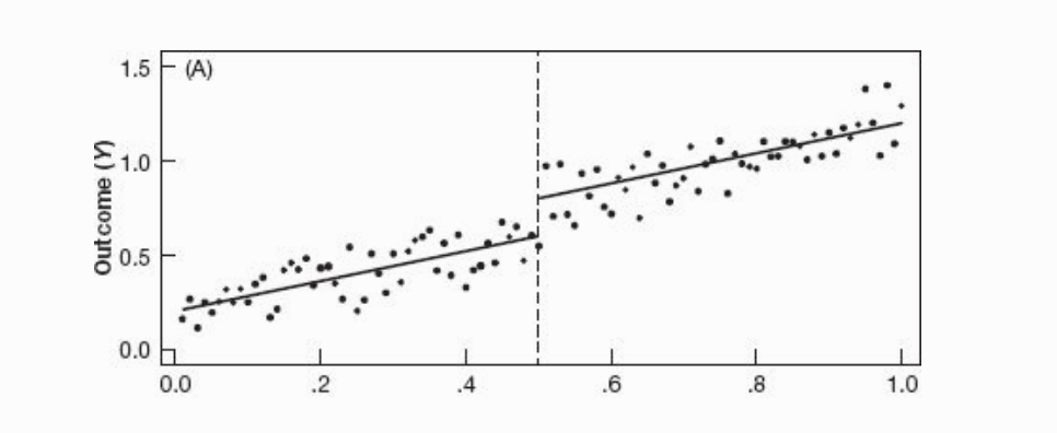
Source: Mostly Harmless Econometrics An Empiricist’s Companion by Joshua Angrist and Jorn-Steffen Pischke
The primary assumptions in this case are twofold. First, the status of the treatment is a deterministic function of the cut off. This means that there is no way to get around the cutoff, it is the sole determinant of access to the treatment. Second, the treatment is discontinuous. This means that even if an individual is arbitrarily close to the cut off on either side, the individual will clearly fall into one group or the other.
Since things aren’t perfect, especially so in the world of causal inference, cases exist where there is no sharp regression discontinuity. This happens because people who get selected in either the treatment or control group around the neighborhood of the cutoff might be non compliant and find a way to move to the other group. As a result, the treatment and control are not cleanly assigned to two groups as in the case of the sharp regression discontinuity. However, what does happen and can be used to draw causal inference is the fact that the probability of being treated is higher on one side of the cut off and lower on the other side of the cut off. Economists call this situation a fuzzy regression discontinuity.
To estimate the causal effect of the treatment an instrumental variable design using two stage least squares is used. The instrument in this case is a dummy variable (0 or 1) assigned to each individual according to the actual cutoff. The estimation of the causal effect is in two stages. The first stage regresses the actual treatment that ends up being assigned after non compliance on the dummy variable assigned by the cutoff. This estimates, in loose terms, the probability of receiving the treatment given the actual cutoff. The second stage regresses the outcome variable of interest on this predicted value of the the intensity of the treatment. The coefficient on this is interpreted as the causal effect of the treatment.
A good question to ask is why the cutoff dummy is a valid instrument for the treatment. This can be argued based on two facts about the cutoff that satisfy the selection conditions of a valid instrument. First, the cutoff is a randomly assigned or arbitrary, there is no selection problem in the assignment of the cut off. Second, the cutoff as an instrument also satisfies the exclusion restriction; i.e., the only way in which it affects the outcome variable of interest is via the treatment.
If you’re interested and getting deeper into the mathematics of how these ideas work, the go to book is Mostly Harmless Econometrics An Empiricist’s Companion by Joshua Angrist and Jorn-Steffen Pischke. For a more math-light treatment of the same ideas, the book to refer is Mastering ‘Metrics: The Path from Cause to Effect by the same authors.